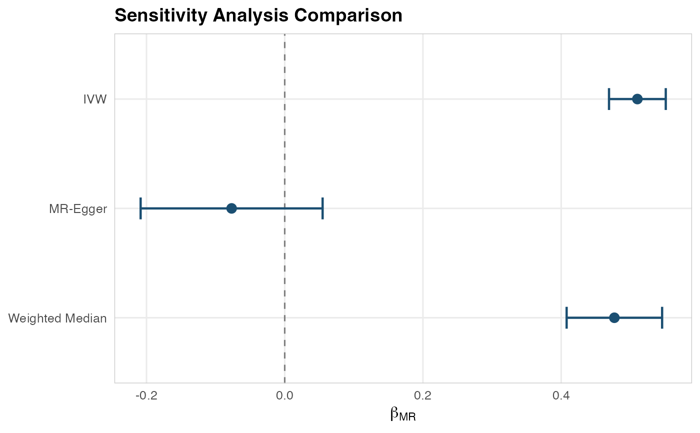
Forest plot comparing MR methods

Creates a horizontal forest plot showing estimates from all sensitivity analysis methods side by side with confidence intervals.

Usage

plotSensitivityForest(sensitivityResults)

Arguments

sensitivityResults

Output of runSensitivityAnalyses.

Value

A ggplot2 object.

Details

Plot Sensitivity Analysis Forest Plot

Examples

set.seed(42)
nSnps <- 10
perSnp <- data.frame(
  snp_id = paste0("rs", 1:nSnps),
  effect_allele = rep(c("A", "C", "G", "T", "A"), length.out = nSnps),
  other_allele = rep(c("C", "G", "T", "A", "C"), length.out = nSnps),
  eaf = seq(0.1, 0.7, length.out = nSnps),
  beta_ZY = rnorm(nSnps, 0.15, 0.02),
  se_ZY = rep(0.02, nSnps),
  beta_ZX = rnorm(nSnps, 0.3, 0.05),
  se_ZX = rep(0.05, nSnps)
)
results <- runSensitivityAnalyses(perSnp, engine = "internal")
#> Running sensitivity analyses with 10 SNPs...
#>   Engine: internal
#>   IVW...
#>   MR-Egger...
#>   Weighted Median...
#>   Steiger filtering...
#> Warning: Steiger filtering is not implemented for binary outcomes because logistic-regression coefficients cannot be converted to correlations without additional scale assumptions. Returning NA result.
#>   Leave-One-Out...
#> Sensitivity analyses complete.
plotSensitivityForest(results)
#> `height` was translated to `width`.